
A Bridge on Economic Issues between China and the World



 Facebook
  Twitter
  Instagram
 WeChat
  Email
Email When Do Financial Frictions Matter for Misallocation?
Financial frictions are often viewed as a key source of misallocation in developing economies, but their quantitative importance is still debated. Firm-level data from China point to large and persistent capital distortions, which are strongly correlated with financial frictions. A quantitative heterogeneous firm model suggests that eliminating financial frictions can generate large productivity gains when other, nonfinancial sources of capital distortion are also present.

A large body of literature following Hsieh and Klenow (2009) has documented substantial capital misallocation in developing economies such as China. A natural explanation is underdeveloped financial markets: if firms cannot borrow freely, capital may fail to flow to its most productive uses. Yet despite this intuition, the quantitative importance of financial frictions remains highly debated.
On one side, influential studies by Midrigan and Xu (2014) and Moll (2014) argue that canonical financial frictions generate only modest productivity losses. In these models, constrained firms can accumulate internal funds over time and eventually grow out of their borrowing constraints. On the other side, work by Buera et al. (2011) and Song et al. (2011) finds that financial frictions play a central role in shaping resource allocation and aggregate productivity.
This divergence raises a fundamental question: When and under what conditions do financial frictions matter quantitatively for misallocation?
A new empirical fact: Borrowing costs and capital distortions are highly correlated in China
Building on this literature, our recent work (Bai et al. 2026) provides new firm-level evidence to examine the relationship between capital misallocation and financial frictions.
A standard measure of capital misallocation is the dispersion in the average revenue product of capital (ARPK): In an efficient allocation, all firms should have the same marginal return to capital. Large dispersion thus signals misallocation. We use ARPK to approximate the marginal return to capital: firms with high ARPK tend to operate with too little capital, and firms with low ARPK have too much capital.
Additionally, we use firm-level average borrowing costs to proxy for firms’ financial conditions, in the spirit of Gilchrist et al. (2013). Borrowing costs are measured as total interest payments divided by fixed assets. A firm with higher borrowing costs suggests a worse financial condition. Note that this measures realized borrowing costs rather than the shadow marginal cost of borrowing, which cannot be directly observed from the data.
We first look into the US, the country with the most developed financial market. Using Compustat data for US manufacturing firms, we find that borrowing costs are weakly correlated with ARPK (Figure 1). This pattern is consistent with the prediction of a model where financial frictions play a small role in capital misallocation, in line with the view that the US economy is highly financially developed. It is also consistent with Gilchrist et al. (2013), who find that the observed dispersion in borrowing costs of US manufacturing firms implies little misallocation.
On the other hand, when using Chinese manufacturing firm-level data, we find that China has much larger dispersion in both borrowing costs and ARPK. Moreover, we uncover a significant correlation: firms with higher ARPK (those that appear more capital-constrained) also face higher borrowing costs (Figure 1). This positive relationship is robust across time, ownership types, and specifications. It is also largely driven by persistent firm-level differences.
Such strong correlation in China aligns with the prediction of a model where financial frictions are strong: firms with higher ARPK are unable to expand due to financial frictions, as reflected in their higher borrowing costs. This finding suggests that, although financial frictions are weak in the US, they can potentially play a large role in misallocation in China.
Figure 1: Borrowing Costs and ln(ARPK) in China and the US
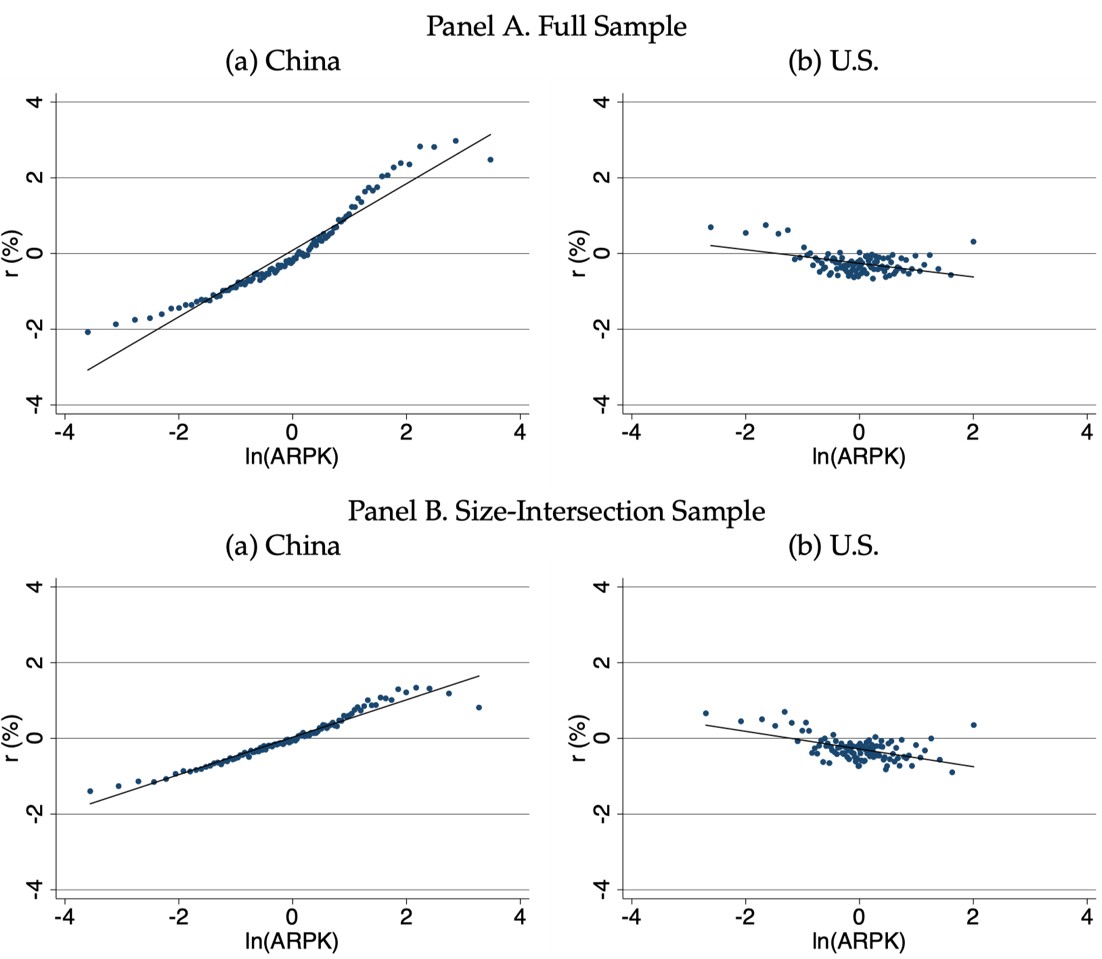
Note: This figure shows the scatter plot of borrowing costs against ln(ARPK) for Chinese and US Compustat manufacturing firms. Both variables are demeaned at the year-by-industry level. For each year, firms are grouped into 100 percentiles of ln(ARPK), and the mean values of borrowing costs and ln(ARPK) are computed within each percentile. The scatter plot represents the average across years from 1998 to 2007. The solid line depicts the fitted linear relationship. Panel A shows results using each country’s full sample, while Panel B shows results based on the intersection sample by asset size between the two countries. Data sources: Chinese manufacturing firm-level data and US Compustat manufacturing data, averaged over 1998–2007.
Financial frictions matter for misallocation when they interact with other distortions
Motivated by the empirical findings, we construct heterogeneous firm models to quantify the extent to which financial frictions matter for misallocation in China.
First, we construct a model with canonical financial frictions, following Khan et al. (2014) and Ottonello and Winberry (2020). The canonical financial frictions are modelled along two dimensions: firms cannot issue new equity, and their only source of external financing is state-noncontingent debt (whose required payments do not vary with firm outcomes) with the option to default. State-noncontingent debt arises from asymmetric information, and endogenous default reflects limited enforcement—these are the two fundamental sources of market incompleteness underlying the financial frictions. The model is calibrated to match Chinese firms’ financing patterns of borrowing costs and leverage.
This model suggests that eliminating financial frictions increases TFP by less than 0.4% (Figure 3, No Exogenous Wedges). This small number is consistent with Midrigan and Xu (2014) and Moll (2014), who find that financial frictions matter little for misallocation. However, as shown in Panel B of Figure 2, the model has two discrepancies from the data: although borrowing costs are positively correlated with ln(ARPK) this model generates much smaller dispersion in ln(ARPK) than in the data; the dispersion in borrowing costs is driven primarily by a small mass of firms—roughly 1%—that face extremely high borrowing costs, while the majority of firms face relatively low borrowing costs in the model.
Figure 2: Borrowing Costs and ln(ARPK) : Model vs. Data
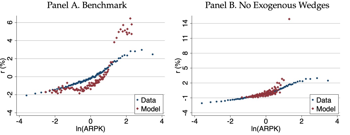
Note: This figure shows the scatter plot of borrowing costs against ln(ARPK). Both variables are demeaned at the year-by-industry level. For each year, firms are grouped into 100 percentiles of ln(ARPK), and the mean values of the borrowing cost and ln(ARPK) are computed within each percentile. The blue round markers represent Chinese manufacturing firms, and the scatter plot reflects the average across years from 1998 to 2007. The red diamond markers represent model simulations of 10,000 firms over 500 periods starting from the stationary equilibrium, and the plotted points are averaged over all simulated periods. Model variables are demeaned at the year level. The left panel shows results from the benchmark model, while the right panel shows the reference model without exogenous wedges (recalibrated). Data sources: Chinese manufacturing firm-level data, averaged over 1998–2007.
Given these discrepancies, we develop a model with not only the canonical financial frictions but also persistent firm-level distortions, or “exogenous wedges,” that capture factors such as regulatory policies, preferential treatment, or institutional differences across firms. We use to denote the wedges on firms’ output: τ > 1 acts as an implicit tax, whereas τ < 1 acts as an implicit subsidy. Now, the model can be calibrated to match both firms' financing patterns and the dispersion in ARPK through the exogenous wedges, which greatly improves the model's fit to the data (Panel A of Figure 2).
In the presence of these distortions, financial frictions become much more distortionary. As shown in Figure 3, when financial frictions interact with exogenous wedges, eliminating financial frictions raises total factor productivity by about 25%.
Figure 3: Total Factor Productivity (TFP) Loss Decomposition
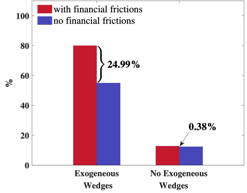
Note: This figure shows TFP losses across model specifications. The left two bars correspond to the model with exogenous wedges, while the right two bars correspond to the model without exogenous wedges. The numbers above the bars report TFP losses relative to their respective efficient TFP levels in log points. The red bars represent the baseline models with financial frictions. The blue bars represent counterfactuals in which financial frictions are shut down.
This large difference arises because the interaction between financial frictions and wedges generates persistent and endogenous financial heterogeneity across firms.
First, introducing exogenous wedges adds another dimension of heterogeneity. Taxed firms face tighter effective financial constraints than subsidized firms, as shown in Panel A of Figure 4. Moreover, tax-like wedges prevent even highly productive firms from expanding to their efficient scale. These firms remain small and asset-poor, which increases their default risk and raises their borrowing costs. As a result, productive firms can remain persistently financially constrained, rather than growing out of those constraints.
Figure 4: Endogenous Financial Heterogeneity
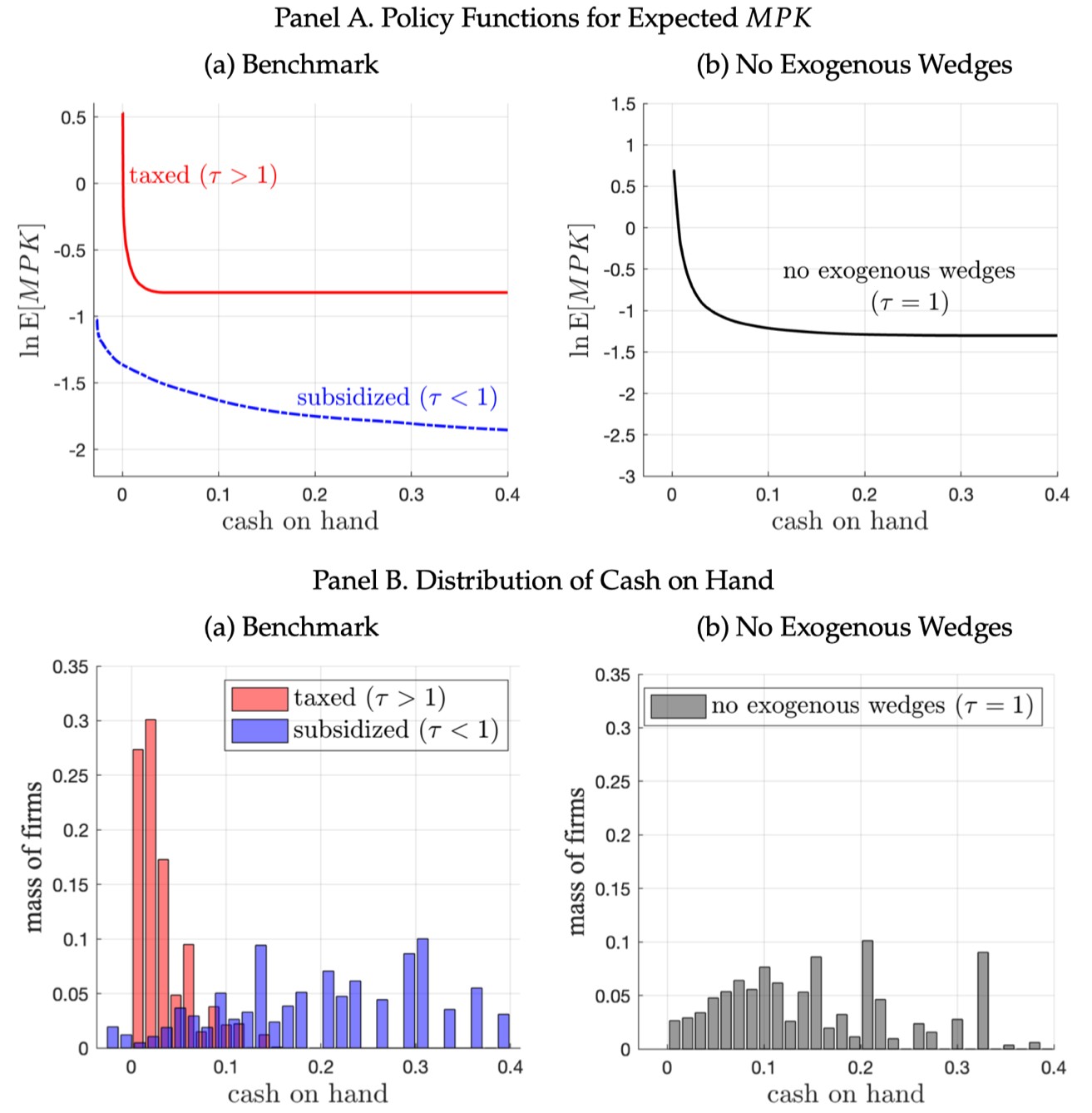
Note: This figure illustrates how exogenous wedges generate endogenous financial heterogeneity. Panel A displays the policy functions for ln E[MPK] of median-productivity firms as a function of cash on hand. Panel B presents the corresponding stationary distribution of cash on hand, also for median-productivity firms. In both panels, the left subplots correspond to the benchmark model with exogenous wedges, where red represents taxed firms (τ > 1) and blue represents subsidized firms (τ < 1). The right subplots show the recalibrated reference model without exogenous wedges (i.e., τ = 1 for all firms).
Second, endogenous selection reinforces this mechanism. Among firms facing high distortions, only the most productive survive (Figure 5). These surviving firms have high returns to capital but also face tight financial constraints, further amplifying misallocation. Without exogenous wedges, selection operates only through productivity, and this channel is quantitatively weak because firms can largely self-finance.
Figure 5: Ex-Post Joint Distribution of Exogenous Wedges and Productivity
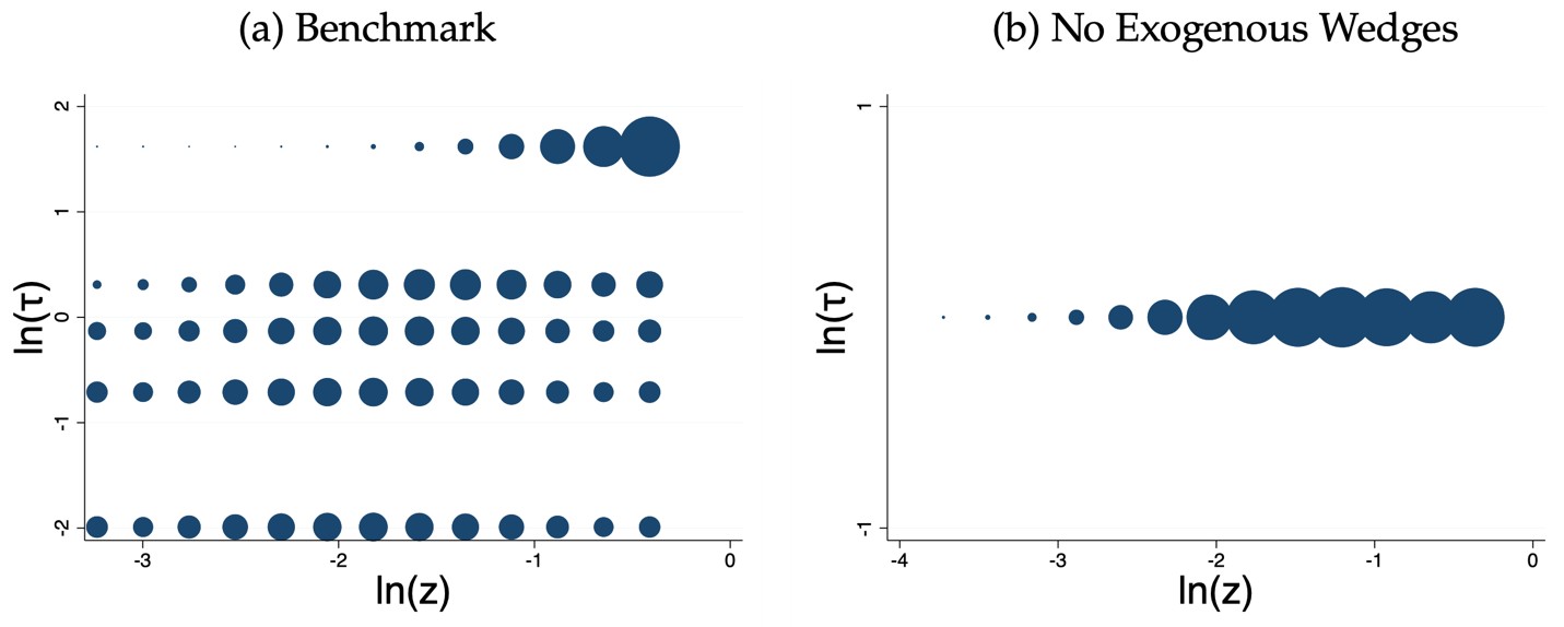
Note: This figure shows the ex-post joint distribution of exogenous wedges (τ) and productivity (z) in the stationary equilibrium, where each dot represents the mass of firms. The left subplot corresponds to the benchmark model with exogenous wedges, while the right subplot shows the recalibrated reference model without exogenous wedges (i.e., τ = 1 for all firms).
Conclusion
Our findings help reconcile the mixed conclusions in the literature. Financial frictions can appear quantitatively unimportant in isolation, but they become highly distortionary when they interact with persistent firm-level distortions.
This suggests that a key difference between developing and developed economies lies not only in the severity of financial frictions, but also in the presence of other distortions that interact with them. Addressing misallocation therefore requires going beyond financial reforms alone.
References
Bai, Yan, Dan Lu, Xu Tian, and Yajie Wang. 2026. “When Do Financial Frictions Matter for Misallocation?” National Bureau of Economic Research Working Paper No. 34930. https://www.nber.org/papers/w34930.
Buera, Francisco J., Joseph P. Kaboski, and Yongseok Shin. 2011. “Finance and Development: A Tale of Two Sectors.” American Economic Review 101 (5): 1964–2002. https://doi.org/10.1257/aer.101.5.1964.
Gilchrist, Simon, Jae W. Sim, and Egon Zakrajšek. 2013. “Misallocation and Financial Market Frictions: Some Direct Evidence from the Dispersion in Borrowing Costs.” Review of Economic Dynamics 16 (1): 159–76. https://doi.org/10.1016/j.red.2012.11.001.
Hsieh, Chang-Tai, and Peter J. Klenow. 2009. “Misallocation and Manufacturing TFP in China and India.” Quarterly Journal of Economics 124 (4): 1403–48. https://doi.org/10.1162/qjec.2009.124.4.1403.
Khan, Aubhik, Tatsuro Senga, and Julia K. Thomas. 2020. “Default Risk and Aggregate Fluctuations in an Economy with Production Heterogeneity.” https://juliathomas.net/KSTdefaultFeb2020.pdf
Midrigan, Virgiliu, and Daniel Yi Xu. 2014. “Finance and Misallocation: Evidence from Plant-Level Data.” American Economic Review 104 (2): 422–58. https://doi.org/10.1257/aer.104.2.422.
Moll, Benjamin. 2014. “Productivity Losses from Financial Frictions: Can Self-Financing Undo Capital Misallocation?” American Economic Review 104 (10): 3186–3221. https://doi.org/10.1257/aer.104.10.3186.
Ottonello, Pablo, and Thomas Winberry. 2020. “Financial Heterogeneity and the Investment Channel of Monetary Policy.” Econometrica 88 (6): 2473–2502. https://doi.org/10.3982/ECTA15949.
Song, Zheng, Kjetil Storesletten, and Fabrizio Zilibotti. 2011. “Growing like China.” American Economic Review 101 (1): 196–233. https://doi.org/10.1257/aer.101.1.196.

Latest
Most Popular
- VoxChina Covid-19 Forum (Second Edition): China’s Post-Lockdown Economic Recovery VoxChina, Apr 18, 2020
- China’s Great Housing Boom Kaiji Chen, Yi Wen, Oct 11, 2017
- China’s Joint Venture Policy and the International Transfer of Technology Kun Jiang, Wolfgang Keller, Larry D. Qiu, William Ridley, Feb 06, 2019
- The Dark Side of the Chinese Fiscal Stimulus: Evidence from Local Government Debt Yi Huang, Marco Pagano, Ugo Panizza, Jun 28, 2017
- Wealth Redistribution in the Chinese Stock Market: the Role of Bubbles and Crashes Li An, Jiangze Bian, Dong Lou, Donghui Shi, Jul 01, 2020
- Evaluating Risk across Chinese Housing Markets Yongheng Deng, Joseph Gyourko, Jing Wu, Aug 02, 2017
- Daily Price Limits and the Magnet Effect Ting Chen, Zhenyu Gao, Jibao He, Wenxi Jiang, Wei Xiong, Oct 25, 2017
- What Is Special about China’s Housing Boom? Edward L. Glaeser, Wei Huang, Yueran Ma, Andrei Shleifer, Jun 20, 2017
- Privatization and Productivity in China Yuyu Chen, Mitsuru Igami, Masayuki Sawada, Mo Xiao, Jan 31, 2018
- How did China Move Up the Global Value Chains? Hiau Looi Kee, Heiwai Tang, Aug 30, 2017