Local fiscal policies have been very effective in China since 2000. At the prefecture city level between 2001 and 2019, the present value of accumulated real GDP is estimated to have increased by 11.4 RMB when government spending increased by 1 RMB on the margin. The large marginal effect can be explained by the high demand for public investment and the presence of government financial constraints that limit local governments’ ability to take all the efficient investment opportunities.

Despite local officials’ strong political incentive to promote economic growth through local fiscal policies in China (Maskin, Qian, and Xu 2000; Xiong 2018), little empirical work has been done to evaluate the effectiveness of these policies. Interest in the macroeconomic effect of fiscal policies has also grown worldwide since the Global Financial Crisis. I provide the first model-free evaluation of local fiscal policies in China since 2000 by estimating the local government spending multiplier, i.e., how much the local GDP increased when local government spending increased by 1 RMB.

To estimate the local government spending multiplier, one must address the endogeneity of local government spending. One cannot simply regress GDP on local government spending and interpret the coefficient as the multiplier because the causality may go the other way and other factors may affect both GDP and government spending. I develop a novel instrument for local government spending after 2000 using the fraction of unoccupied raw land in each city’s downtown area in 2000. After 2000, as the market for land was formalized and land sale revenue became an important source of income for local governments, a higher fraction of unoccupied raw land implied less required compensation expense to pre-occupants displaced from the land and hence higher net profits of land sales for local governments.

With the rise of the land market, the fraction of unoccupied raw land led to exogenous variation of local government spending. It is exogenous because in 2000, it was not significantly correlated with either the level or the growth of various local economic variables (e.g., GDP, number of manufacturing firms, urban employment), government spending (e.g., budgetary expenditures and revenues, infrastructure investment), initial level of infrastructures (e.g., road area, length of water supply and drainage pipelines), local firm characteristics, land supply, or land zoning. It appears that in 2000, when land value was low, local governments left unoccupied land, such as rivers and lakes, as they were. After 2000, when land value became high, governments began making better use of unoccupied land by, for example, filling rivers and lakes to transform them into usable land. Moreover, the fraction of raw land did not affect future economic growth through other channels, such as net land supply, the cyclicality of local economy and construction, or pick up other shocks such as the city’s exposure to WTO accession. Therefore, the fraction of unoccupied raw land can be used as an instrument variable to study the causal effect of local government spending on GDP.

Using the fraction of unoccupied land as the exogenous shock to government spending, I estimate the impulse responses of local GDP and government spending. The multiplier is the ratio of the present value of the impulse responses of the local GDP and government spending. Figure 1 shows the multiplier for each horizon. The multiplier increases over time and converges to about 11. In 2019, it was estimated to be 11.4, with the 95% confidence interval between 7.1 and 15.6. The increasing trend suggests the persistent effect of government spending. With persistent effect, we capture more of the effect of government spending occurred in the early years as we move along the horizon.

The multiplier is typically found to be much smaller in other countries. Chodorow-Reich (2019) reviewed recent literature and concluded that the preferred estimate in the US is 1.8. For India, Jain and Kumar (2013) found the multiplier to be 1.07. For low-income countries, Kraay (2012) found the multiplier to be only 0.5. In general, the multiplier tends to be smaller in less-developed countries.

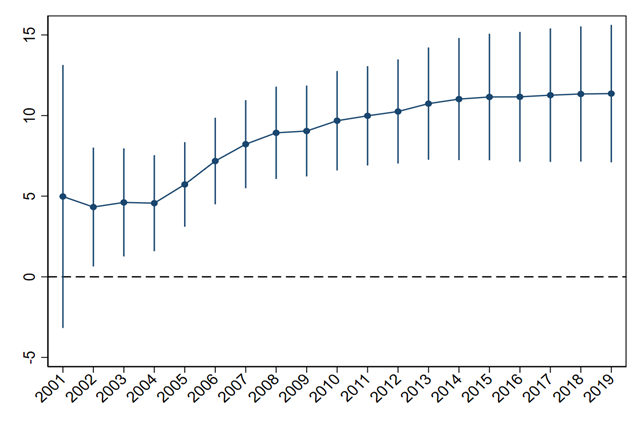
Figure 1: Estimated Local Government Spending Multiplier over time

So, why is the local government spending multiplier so much larger in China? Conceptually, a high multiplier can exist in an equilibrium where the government has good investment opportunities but is financially constrained from seizing on those opportunities. Under such equilibrium, a marginal increase in government spending can have a large effect. Under the alternative equilibrium where the government has perfect access to outside financing or relatively few investment opportunities, it could take all the investment opportunities, and the additional money, such as grants from federal governments, would be spent more on government consumption and would generate a smaller marginal effect on output. In the US after 2000, with most infrastructure already in place and the presence of the municipal bond market to finance additional investment if needed, any fiscal stimulus was mostly spent on non-infrastructure expenditures and generated a small impact on output. Before 2000, demand for new investment may have been relatively high but there was no systematic estimation of the government general spending multiplier. David Alan Aschauer was among the few researchers who found a large multiplier (about 13) for government infrastructure investment. For other developing countries, the multiplier was found to be small, as low economic growth led to low demand for government investment or was associated with low efficiency of the budgetary system.

Consistent with the hypothesis of financial constraint, I find the multiplier to be significantly smaller in cities that have better access to outside debt financing, which is defined as a higher average debt-to-income ratio after 2000. The significant difference survives despite the possibility that a higher debt-to-income ratio might be associated with better investment opportunities, which should imply a higher multiplier. In terms of magnitude, for the half cities with higher debt-to-income ratio, the multiplier is estimated to be 1. For the role of investment opportunities, the multiplier is found to be significantly higher in cities that benefit more from China’s entry into WTO in 2001 measured with their export growth, and in cities with worse infrastructure in 2000 measured with their total road area.

To have a better sense of how much local government spending loads on infrastructure, I estimate the marginal propensity to spend on infrastructure, which is the marginal increase of infrastructure investment when total spending increases by 1 RMB, to be about 0.5 in the early years following 2000. It decreased gradually over time and was about 0.2 in 2019. Other categories of spending, although likely not as productive as infrastructure investment, also could have benefited the local economy as they might have, for example, helped attract skilled laborers and improve local business conditions.

Overall, government spending has also behaved like investment. The increase of government spending is found to increase local labor demand as both employment and wages increased. Over time, as people moved to cities with higher wages, the wage gap closed in later years while the employment gap kept increasing. Government spending is also found to crowd-in private investment in the form of firm entry. The persistency of firm entry explains the persistency of the effect of government spending. What’s more, local firms’ productivity and market access also increased, especially for those that used more transportation services.

Local government spending has also generated positive spillovers across different regions within the same city through technology diffusion and supply-chain linkages. But there is no evidence of spillovers on neighboring cities. The lack of spillovers in the dimension of geographic distance, however, does not necessarily mean that we can equate the local multiplier to the national multiplier, because there may be spillovers in other dimensions. For example, since one main effect of government spending is to attract entrants, two cities with similar industry structure may be direct competitors. Estimating the nationwide government spending multiplier is beyond the scope of this work. There is still much research to be done in the future to understand how local fiscal policies have contributed to China’s total economic growth.

References

Chodorow-Reich, Gabriel. 2019. “Geographic Cross-Sectional Fiscal Spending Multipliers: What Have We Learned?” American Economic Journal: Economic Policy 11(2): 1–34. https://doi.org/10.1257/pol.20160465.

Jain, Rajeev, and Prabhat Kumar. 2013. “Size of Government Expenditure Multipliers in India: A Structural VAR Analysis.” Reserve Bank of India Working Paper Series No. 7. https://rbi.org.in/scripts/PublicationsView.aspx?Id=15369.

Kraay, Aart. 2012. “How Large Is the Government Spending Multiplier? Evidence from World Bank Lending.” Quarterly Journal of Economics 127(2): 829–87. https://doi.org/10.1596/1813-9450-5500.

Maskin, Eric, Yingyi Qian, and Chenggang Xu. 2000. “Incentives, Information, and Organizational Form.” Review of Economic Studies 67(2): 359–78. https://doi.org/10.1111/1467-937X.00135.

Ramey, Valerie A. 2020. “The Macroeconomic Consequences of Infrastructure Investment.” NBER Working Paper No. 27625. https://doi.org/10.3386/w27625.

Xiong, Wei. 2018. “The Mandarin Model of Growth.” NBER Working Paper No. 25926. https://doi.org/10.3386/w25296.